Building a “Propensity to Convert” machine learning model with Snowpark and Snowplow web tracking – Part one
When a user first visits a website or application, you can begin to track their behavior. This behavior, however limited during a first visit, can then be used to predict their future actions.
One possible future action is a ‘conversion’, which could be defined as a purchase, sign-up, or subscription (amongst many, many other things). Understanding how likely a user us to ‘convert’ is invaluable to digital companies because it allows marketers to:
- Assess the effectiveness of different digital ad campaigns – especially where the users acquired might not have converted. However, it is already possible (based on their data) to predict that many are likely to.
- Identify an audience for retargeting; i.e. focus ad spend on those users who are likely to convert (and save money by not reacquiring users who are not likely to convert).
- Understand what parts of a user’s initial experience predict their conversion and what parts in the user journey are essential.
- Identify parts of the user journey that did not get as much attention as needed. For example, time spent browsing documentation is predictive, but the marketing team has neglected to invest in documentation, not realizing its critical role in driving conversion. It might highlight that some experiences make the user less likely to convert, and these need to be dealt with urgently.
First-touch attribution
The first touch approach to marketing attribution states that all credit for the user conversion goes to the first advertisement on the user journey. Last-touch attribution, on the other hand, assigns all credit to the last advertisement, whereas multi-touch attribution takes into account all interactions along the user journey.
First-touch attribution is less common than last- or multi-touch attribution [1], [2], and is generally used to measure the effectiveness of brand building campaigns or to assign credit in short sales cycles.
The following guide explores the impact of measuringbehavioral data during initial contact with the website on propensity model accuracy. The impact of these statistics is less researched since most web trackers do not collect them; i.e., Google Ad Campaign [3].
Snowplow for attribution
Snowplow web tracking includes engagement metrics out of the box:
- Scroll depth
- Engaged time (with page)
- Time tab open in browser
Other standard features of the out-of-the box trackers include referral source, temporal markers, marketing campaign ID, geo-data, and device details.
Modeling for churn propensity
Marketing teams need to identify the reasons behind projected conversions, which means that model interpretability is incredibly important. Because of this, we have to put limits on feature preprocessing methods and classifiers; algorithms that aggregate features during preprocessing (such as PCA), for example, will render feature importance unusable.
The chosen baseline is Logistic Regression [4], the most researched and widely spread in marketing attribution. Gradient Boosting Trees with LightGBM [5] often perform better than neural networks or linear models for highly categorical data sets. It also offers explainability through the decision tree visualization and SHAP TreeExplainer (after the number of features had been cut down)
Dataset
The dataset in the example below has been taken from snowplow.io, which receives hundreds of thousands of visitors annually. Less than 0.5% of total visitors convert into prospects via the demo request form.
Users are tracked by the cookies set when they initially visit the website. Of course, when the user clears the cookies, does not accept the cookie disclaimer or logs through a different device, this information is lost, resulting in multiple rows per the same user. Snowplow’s dbt web user model performs aggregation by cookies.[7]
Model features could be grouped into categories based on their origin:
- Temporal – created from first event timestamp: an hour of the day, day of the week.
- Landing Page – page title of the first URL, comes out of the box
- Device – User Agent enrichment [8]
- Referral – Referral enrichment[9]
- Marketing – Marketing campaign enrichment[10]
- Geographic – IP lookup enrichment[11]
- Robot – IAB enrichment[12]
- Engagement – Accumulated page ping events by dbt page view model [13].
Conversion events are taken from Salesforce, using different tracking methods. However, in practice Snowplow users could send a custom conversion event to avoid joining another data source. Read our documentation about setting this up [14].
Snowplow has been able to deliver high-quality behavioral data to Snowflake since earlier this year (2022). For this research, earlier data kept in Redshift had been partially migrated into Snowflake.
Most recent data should not be considered for the performance as some users have not converted yet. (The purchase cycle for Snowplow BDP can be long.)
Data preprocessing with Snowpark
Snowflake has released a limited access version of the Snowplow park python library (with the full version to be released soon. This library allows you to work with snowflake data as lazily evaluated DataFrame classes with an interface similar to pyspark DaraFrames; it has complete SQL functionality, with some additional features on top. It’s very easy to learn and would be familiar with SQL or Panda users (I was able to pick this up in a week).
There are a few essential imports and jupyter notebook style settings required initially.
import datetime

import imblearn.pipeline
import pandas as pd
import numpy as np
from matplotlib import pyplot as plt
from IPython.core.display import HTML
from IPython.core.display_functions import display

display(HTML("<style>pre { white-space: pre !important; }</style>"))
pd.options.display.max_columns = None
pd.options.display.max_rows = None
First, a session should be established for the snowflake instance.
from snowflake.snowpark import Session

with open("pavel-snowflake-dev.properties") as file:
    props = dict([l.rstrip().split(" = ", 2) for l in file.readlines() if " = " in l])

session = Session.builder.configs(props).create()
session.sql("ALTER SESSION SET TIMEZONE = 'UTC';");
Template of pavel-snowflake-dev.properties file:
account = XXXXXX
region = eu-west-1
user = USER
password = ********
DATABASE = DBNAME
schema = SCHEMA_NAME
warehouse = WHNAME
role = ROLE
Data comes from multiple sources. Historic data had been imported into Snowflake from our old Redshift instance. To reduce the volume of transferred data we have already joined the users and page_views in the historic tables.
The users dbt model had been slightly customized, adding the first session of each user, which is just an extra field alongside the already existing FIRST_PAGE_TITLE the FIRST_PAGE_VIEW_ID. This makes it easier to join users with the page_views.
CONVERTED_DATE field had been added by joining the custom conversion event with the Salesforce data.
So our four data sources are defined (see the schemas and description of each field in the snowplow dbt web model docs):
users_df = session.table("ANALYTICS_DEV_DB.DBT_EMIEL_DERIVED.SNOWPLOW_WEB_USERS")
page_view_df = session.table("ANALYTICS_DEV_DB.DBT_EMIEL_DERIVED.SNOWPLOW_WEB_PAGE_VIEWS")
rs2021_df = session.table("ANALYTICS_DEV_DB.DBT_EMIEL_DERIVED.REDSHIFT_FEATURES_2021")
rs2020_df = session.table("ANALYTICS_DEV_DB.DBT_EMIEL_DERIVED.REDSHIFT_FEATURES_2020")
Next all our sources of data are joined together. Note, how Snowpark DataFrame calls could be chained into the code that closely resembles an SQL statement. The result is the list of primary features before preprocessing.
from snowflake.snowpark.functions import coalesce, timestamp_ntz_from_parts, dayofmonth, year, month, minute, second, hour

combined_df = users_df\
    .join(page_view_df, page_view_df.PAGE_VIEW_ID == users_df.FIRST_PAGE_VIEW_ID)\
    .join(rs2021_df, rs2021_df.DOMAIN_USERID == users_df.DOMAIN_USERID, join_type='full')\
    .join(rs2020_df, rs2020_df.DOMAIN_USERID == users_df.DOMAIN_USERID, join_type='full').select([
    coalesce(rs2021_df.START_TSTAMP, rs2020_df.START_TSTAMP, users_df.START_TSTAMP).as_("START_TSTAMP"),
    coalesce(rs2021_df.REFR_URLHOST, rs2020_df.REFR_URLHOST, users_df.REFR_URLHOST).as_("REFR_URLHOST"),
    coalesce(rs2021_df.REFR_MEDIUM, rs2020_df.REFR_MEDIUM, users_df.REFR_MEDIUM).as_("REFR_MEDIUM"),
    coalesce(rs2021_df.REFR_TERM, rs2020_df.REFR_TERM, users_df.REFR_TERM).as_("REFR_TERM"),
    coalesce(rs2021_df.MKT_MEDIUM, rs2020_df.MKT_MEDIUM, users_df.MKT_MEDIUM).as_("MKT_MEDIUM"),
    coalesce(rs2021_df.MKT_SOURCE, rs2020_df.MKT_SOURCE, users_df.MKT_SOURCE).as_("MKT_SOURCE"),
    coalesce(rs2021_df.MKT_TERM, rs2020_df.MKT_TERM, users_df.MKT_TERM).as_("MKT_TERM"),
    coalesce(rs2021_df.MKT_CAMPAIGN, rs2020_df.MKT_CAMPAIGN, users_df.MKT_CAMPAIGN).as_("MKT_CAMPAIGN"),
    coalesce(rs2021_df.MKT_CONTENT, rs2020_df.MKT_CONTENT, users_df.MKT_CONTENT).as_("MKT_CONTENT"),
    coalesce(rs2021_df.MKT_NETWORK, rs2020_df.MKT_NETWORK, users_df.MKT_NETWORK).as_("MKT_NETWORK"),
    coalesce(rs2021_df.GEO_COUNTRY, rs2020_df.GEO_COUNTRY, page_view_df.GEO_COUNTRY).as_("GEO_COUNTRY"),
    coalesce(rs2021_df.GEO_REGION, rs2020_df.GEO_REGION, page_view_df.GEO_REGION).as_("GEO_REGION"),
    coalesce(rs2021_df.BR_LANG, rs2020_df.BR_LANG, page_view_df.BR_LANG).as_("BR_LANG"),
    coalesce(rs2021_df.DEVICE_FAMILY, rs2020_df.DEVICE_FAMILY, page_view_df.DEVICE_FAMILY).as_("DEVICE_FAMILY"),
    coalesce(rs2021_df.OS_FAMILY, rs2020_df.OS_FAMILY, page_view_df.OS_FAMILY).as_("OS_FAMILY"),
    coalesce(rs2021_df.OPERATING_SYSTEM_CLASS, rs2020_df.OPERATING_SYSTEM_CLASS,
             page_view_df.OPERATING_SYSTEM_CLASS).as_(
        "OPERATING_SYSTEM_CLASS"),
    coalesce(rs2021_df.OPERATING_SYSTEM_NAME, rs2020_df.OPERATING_SYSTEM_NAME, page_view_df.OPERATING_SYSTEM_NAME).as_(
        "OPERATING_SYSTEM_NAME"),
    coalesce(rs2021_df.SPIDER_OR_ROBOT, rs2020_df.SPIDER_OR_ROBOT, page_view_df.SPIDER_OR_ROBOT).as_("SPIDER_OR_ROBOT"),
    coalesce(rs2021_df.FIRST_PAGE_TITLE, rs2020_df.FIRST_PAGE_TITLE, users_df.FIRST_PAGE_TITLE).as_(
        "UNSAFE_FIRST_PAGE_TITLE"),
    coalesce(rs2021_df.FIRST_PAGE_URLHOST, rs2020_df.FIRST_PAGE_URLHOST, users_df.FIRST_PAGE_URLHOST).as_(
        "FIRST_PAGE_URLHOST"),
    coalesce(rs2021_df.FIRST_PAGE_URLPATH, rs2020_df.FIRST_PAGE_URLPATH, users_df.FIRST_PAGE_URLPATH).as_(
        "FIRST_PAGE_URLPATH"),
    coalesce(rs2021_df.ENGAGED_TIME_IN_S, rs2020_df.ENGAGED_TIME_IN_S, page_view_df.ENGAGED_TIME_IN_S).as_(
        "ENGAGED_TIME_IN_S"),
    coalesce(rs2021_df.ABSOLUTE_TIME_IN_S, rs2020_df.ABSOLUTE_TIME_IN_S, page_view_df.ABSOLUTE_TIME_IN_S).as_(
        "ABSOLUTE_TIME_IN_S"),
    coalesce(rs2021_df.VERTICAL_PERCENTAGE_SCROLLED, rs2020_df.VERTICAL_PERCENTAGE_SCROLLED,
             page_view_df.VERTICAL_PERCENTAGE_SCROLLED).as_(
        "VERTICAL_PERCENTAGE_SCROLLED"),
    coalesce(timestamp_ntz_from_parts(
        year(users_df.CONVERTED_DATE),
        month(users_df.CONVERTED_DATE),
        dayofmonth(users_df.CONVERTED_DATE),
        hour(users_df.CONVERTED_DATE),
        minute(users_df.CONVERTED_DATE),
        second(users_df.CONVERTED_DATE)
    ), rs2020_df.CONVERTED_DATE, rs2021_df.CONVERTED_DATE).as_("CONVERTED_DATE")
])

print(f"{'Column':30} Type")
print(f"--------------------------------------")
for field in combined_df.schema.fields:
    print(f"{field.name:30} {field.datatype}")
Column                         Type
--------------------------------------
START_TSTAMP                   Timestamp
REFR_URLHOST                   String
REFR_MEDIUM                    String
REFR_TERM                      String
MKT_MEDIUM                     String
MKT_SOURCE                     String
MKT_TERM                       String
MKT_CAMPAIGN                   String
MKT_CONTENT                    String
MKT_NETWORK                    String
GEO_COUNTRY                    String
GEO_REGION                     String
BR_LANG                        String
DEVICE_FAMILY                  String
OS_FAMILY                      String
OPERATING_SYSTEM_CLASS         String
OPERATING_SYSTEM_NAME          String
SPIDER_OR_ROBOT                Boolean
UNSAFE_FIRST_PAGE_TITLE        String
FIRST_PAGE_URLHOST             String
FIRST_PAGE_URLPATH             String
ENGAGED_TIME_IN_S              Long
ABSOLUTE_TIME_IN_S             Long
VERTICAL_PERCENTAGE_SCROLLED   Double
CONVERTED_DATE                 Timestamp
Snowplow data requires very little preparation before the ML pipeline can consume it. But it helps to add a few temporal features: HOUR and DAY_OF_WEEK.
PAGE_TITLE is chosen over URL as the same page could be reached by the different URL. That could be caused by referral URLs, Google Translate or the page could be moved by a web admin to a different address.
Some tracking events do not capture titles, for example, if they serve pdf. For these, it makes sense to replace them with the URL.
All constants must be wrapped in lit, like the empty replacement string in this snippet:
from snowflake.snowpark.functions import concat, dayname, hour, coalesce, is_null, iff, regexp_replace, replace, lit
from snowflake.snowpark.types import StringType
sp_df = combined_df.select(dayname("START_TSTAMP").as_("DAY_OF_WEEK"),
                          hour("START_TSTAMP").as_("HOUR"),
                          (~is_null(combined_df.CONVERTED_DATE)).as_("CONVERTED_USER"),
                          iff(
                              coalesce(combined_df.UNSAFE_FIRST_PAGE_TITLE, lit("")) == "",
                              concat(combined_df.FIRST_PAGE_URLHOST, combined_df.FIRST_PAGE_URLPATH),
                              combined_df.UNSAFE_FIRST_PAGE_TITLE
                          ).as_("FIRST_PAGE_TITLE"),
                          is_null(coalesce("REFR_URLHOST", "REFR_MEDIUM" , "REFR_TERM")).as_("REFR_ANY"),
                          is_null(coalesce("MKT_MEDIUM", "MKT_SOURCE" , "MKT_TERM", "MKT_CAMPAIGN", "MKT_CONTENT", "MKT_NETWORK")).as_("MKT_ANY"),
                          *combined_df.columns
                          ).where(
    iff(is_null(combined_df.CONVERTED_DATE), True, combined_df.CONVERTED_DATE >= combined_df.START_TSTAMP)
).sort(combined_df.START_TSTAMP.asc())
To avoid exposing future information about the conversion, the dataset is split into 10 equal intervals.
from snowflake.snowpark.functions import max, min
begin, end = sp_df.select(min('START_TSTAMP'),max('START_TSTAMP')).collect()[0]
step_duration = (end - begin) / 10

step_names = []
step_full_names = []
step_dates = []
for i in range(4,10):
    cutoff = begin + step_duration * i
    steps_name = f"CONVERTED_RANGE_{cutoff.date()}"
    step_dates.append(cutoff)
    step_names.append(steps_name)
    step_full_names.append(f" {begin + step_duration * (i-1)} from {cutoff.date()} to ")
    sp_df = sp_df.with_column(steps_name, coalesce(sp_df.CONVERTED_DATE > cutoff, lit(False)))
At this point Snowpark DataFrame had not been materialized yet (SQL statement constructed but hasn’t been executed). Column name and types could be inferred before materialization. That is used to define powerful type-dependent transformations. For example, LightGBM requires column names to not have any JSON control characters, and it will also replace spaces with underscores. Most of the features are categorical and will be encoded downstream with OneHotEncoder. So we could define a function to apply to all String columns:
from snowflake.snowpark._internal.type_utils import ColumnOrName
from snowflake.snowpark import Column
from snowflake.snowpark.functions import regexp_replace, replace, substr


def lgbm_trim(col: ColumnOrName) -> Column:
    return substr(replace(
        regexp_replace(col, """[\"\'\b\f\t\r\n\,\]\[\{\}\"\:\\\\]""")
        , " ", "_"), 0, 190).as_(col)
Finally, lgbm_trim function is applied to every text column. This function is about 3-5 times faster when executed within Snowflake than when the pd.DataFrame.str.replace method was executed on the AWS xlarge instance compares to XS Snowflake warehouse.
Data is exported directly into pandas DataFrame. This is done in a single call. Under the hood it transfers apache arrow objects and has less overhead than SQL driver.
%%time
df = sp_df.to_pandas()
df = df.replace("""[\"\'\b\f\t\r\n\,\]\[\{\}\"\:\\\\]""", '', regex=True).replace(" ", '')
df_obj = df.select_dtypes(['object'])
df[df_obj.columns] = df_obj.apply(lambda x: x.str.slice(0, 200))
df.set_index("START_TSTAMP", inplace=True)
CPU times: user 18.7 s, sys: 1.95 s, total: 20.6 s
Wall time: 26.5 s
%%time
sp_df_clean = sp_df.select(
    [lgbm_trim(f.name) if isinstance(f.datatype, StringType) else f.name for f in sp_df.schema.fields])

df = sp_df_clean.to_pandas()

df.set_index("START_TSTAMP", inplace=True)
CPU times: user 3 s, sys: 357 ms, total: 3.35 s
Wall time: 8.55 s
to_pandas infers the pd.DataFrame types during export.
df.dtypes
DAY_OF_WEEK                             object
HOUR                                      int8
CONVERTED_USER                            bool
FIRST_PAGE_TITLE                        object
REFR_ANY                                  bool
MKT_ANY                                   bool
REFR_URLHOST                            object
REFR_MEDIUM                             object
REFR_TERM                               object
MKT_MEDIUM                              object
MKT_SOURCE                              object
MKT_TERM                                object
MKT_CAMPAIGN                            object
MKT_CONTENT                             object
MKT_NETWORK                             object
GEO_COUNTRY                             object
GEO_REGION                              object
BR_LANG                                 object
DEVICE_FAMILY                           object
OS_FAMILY                               object
OPERATING_SYSTEM_CLASS                  object
OPERATING_SYSTEM_NAME                   object
SPIDER_OR_ROBOT                         object
UNSAFE_FIRST_PAGE_TITLE                 object
FIRST_PAGE_URLHOST                      object
FIRST_PAGE_URLPATH                      object
ENGAGED_TIME_IN_S                        int16
ABSOLUTE_TIME_IN_S                       int32
VERTICAL_PERCENTAGE_SCROLLED           float64
CONVERTED_DATE                  datetime64[ns]
CONVERTED_RANGE_2020-12-16                bool
CONVERTED_RANGE_2021-03-14                bool
CONVERTED_RANGE_2021-06-09                bool
CONVERTED_RANGE_2021-09-05                bool
CONVERTED_RANGE_2021-12-02                bool
CONVERTED_RANGE_2022-02-27                bool
dtype: object
Results of the original query could be cached to improve performance of subsequent queries.
sp_df_cached = sp_df_clean.cache_result()
Exploratory Data Analysis
Snowpark could be used to deal with data sets that do not fit in memory of a single machine. Although, this Snowplow set is not this big, basic EDA was done in Snowpark for demonstration.
Another notable mention is Snowflake’s snowpark.DataFrame.sample method which returns a fraction of rows in a table. It was very useful accelerating prototyping in jupiter, but did not make it into this article.
All groups are categorical, except for engagement.
ref_cols = ["REFR_URLHOST", "REFR_MEDIUM", "REFR_TERM", "REFR_ANY"]
mkt_cols = ["MKT_MEDIUM", "MKT_SOURCE", "MKT_TERM", "MKT_CAMPAIGN", "MKT_CONTENT", "MKT_NETWORK", "MKT_ANY"]
geo_cols = ["GEO_COUNTRY", "GEO_REGION", "BR_LANG"]
dev_cols = ["DEVICE_FAMILY", "OS_FAMILY", "OPERATING_SYSTEM_CLASS", "OPERATING_SYSTEM_NAME"]
url_cols = ["FIRST_PAGE_TITLE"]
robot_cols = ["SPIDER_OR_ROBOT"]
calendar_cols = ["DAY_OF_WEEK", "HOUR"]
engagement_cols = ["ENGAGED_TIME_IN_S", "ABSOLUTE_TIME_IN_S", "VERTICAL_PERCENTAGE_SCROLLED"]

discrete_col = ref_cols + mkt_cols + geo_cols + dev_cols + robot_cols + calendar_cols + url_cols
continues_col = engagement_cols
Identifying balance of classes (converted against unconverted population) in our full data set. Again comparing materialised data set against Snowpark. Both took about the same time.
%%time
X = df[discrete_col + continues_col]
y = df.CONVERTED_USER

print(f"Number of users: {y.shape[0]}")
print(f"Number of conversions: {y[y].count()}")
print(f"Percent of conversions: {y[y].count() / y.shape[0] * 100:.3f} %")
Number of users: 659457
Number of conversions: 3120
Percent of conversions: 0.473 %
CPU times: user 256 ms, sys: 150 ms, total: 407 ms
Wall time: 663 ms
%%time
n_conversions = sp_df_cached.where(sp_df.CONVERTED_USER).count()
n_total = sp_df_cached.count()

print(f"Number of users: {n_total}")
print(f"Number of conversions: {n_conversions}")
print(f"Percent of conversions: {n_conversions / n_total * 100:.3f} %")
Number of users: 659457
Number of conversions: 3120
Percent of conversions: 0.473 %
CPU times: user 18.7 ms, sys: 10 µs, total: 18.8 ms
Wall time: 634 ms
It is important to identify if the data got cyclic patterns or other features like gaps or spikes.
from snowflake.snowpark import Window
from snowflake.snowpark.functions import to_date, avg


sp_df_w_date = sp_df_cached.with_column("ts_date", to_date(sp_df_cached.START_TSTAMP)).group_by(
    "ts_date").count().with_column_renamed("COUNT", "ts_count")
window5d = Window.rows_between(-4, Window.CURRENT_ROW).order_by("ts_count")
ma5d = sp_df_w_date.select('ts_date',  avg(sp_df_w_date.ts_count).over(window5d).as_("TS_COUNT_MA5D")).sort(
    "ts_date").na.drop().to_pandas().astype({
    'TS_COUNT_MA5D': 'float',
    'TS_DATE': "datetime64"
}).set_index("TS_DATE").resample('1D').sum().fillna(0)
ma5d.plot(figsize = (13,4), title="5 day conversions moving average")
<matplotlib.axes._subplots.AxesSubplot at 0x7f6b6271a400>
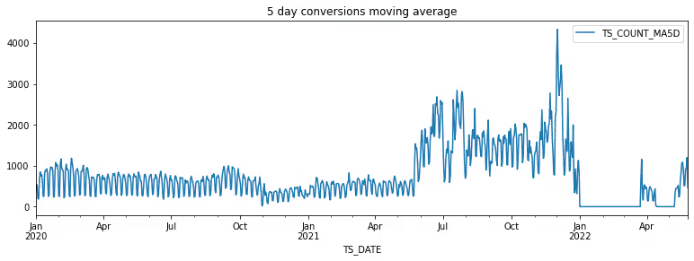
There are a few features of this chart.
- short cyclic trend
- large spikes in December 2021 and around July 2021
- data gap since Jan 2022
It could help to zoom into these areas:
from datetime import date
from matplotlib import pyplot as plt

_, axes = plt.subplots(nrows=4, constrained_layout=True, figsize = (13,12))
ma5d[(date(2020,1,1) <= ma5d.index.date) & (ma5d.index.date < date(2020,2,1))].plot(ax=axes[0], title='Conversions with cyclic trend between 2020-1-1 and 2020-2-1')
ma5d[(date(2021,6,1) <= ma5d.index.date) & (ma5d.index.date < date(2021,8,1))].plot(ax=axes[1], title='Spike of conversions between 2021-6-1 and 2021-6-1')
ma5d[(date(2021,10,1) <= ma5d.index.date) & (ma5d.index.date < date(2022,2,1))].plot(ax=axes[2], title='Conversions with missing data 2021-10-1 and 2022-2-1')
ma5d.tail(100).plot(ax=axes[3])
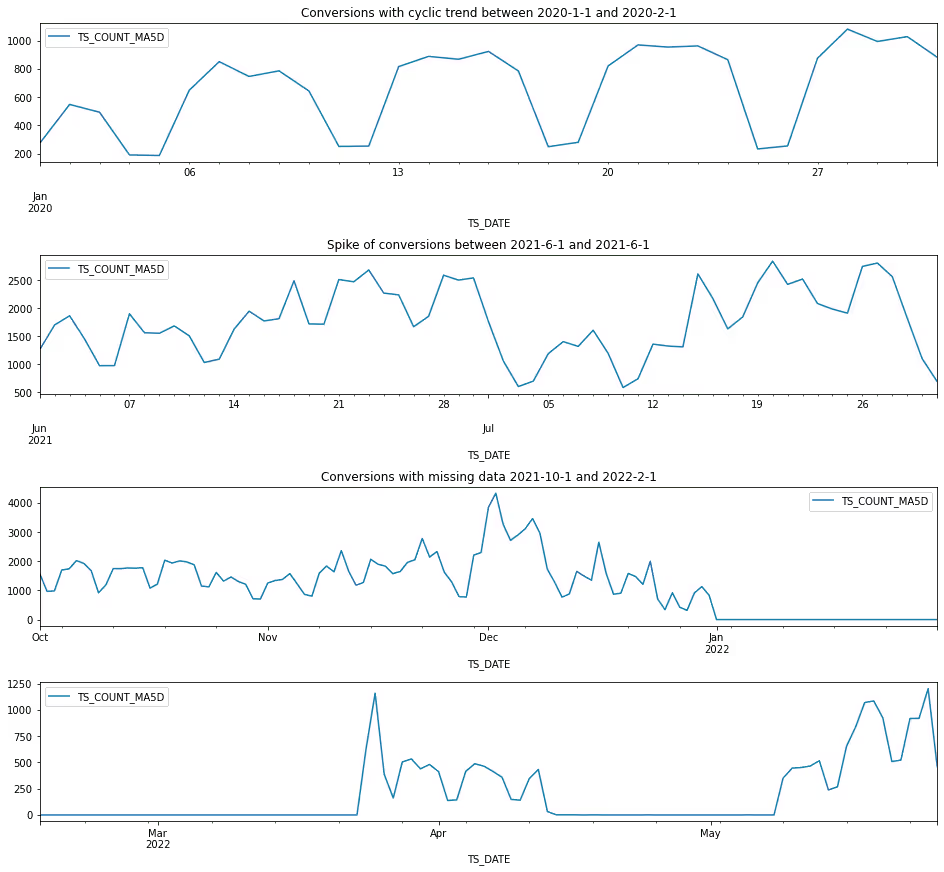
The volume of visitors drops on the weekend, explaining the short cyclic pattern.
Another place of interest is how long visitors take to convert.
from snowflake.snowpark.functions import datediff

data = sp_df_cached.where(sp_df_cached.CONVERTED_USER).select(
    datediff('day',sp_df_cached.START_TSTAMP, sp_df_cached.CONVERTED_DATE).as_("lag")
).to_pandas()

data.plot(bins=100, kind='hist', title = "Conversion lag histogram", figsize=(13,7))
<matplotlib.axes._subplots.AxesSubplot at 0x7f6b62da1280>
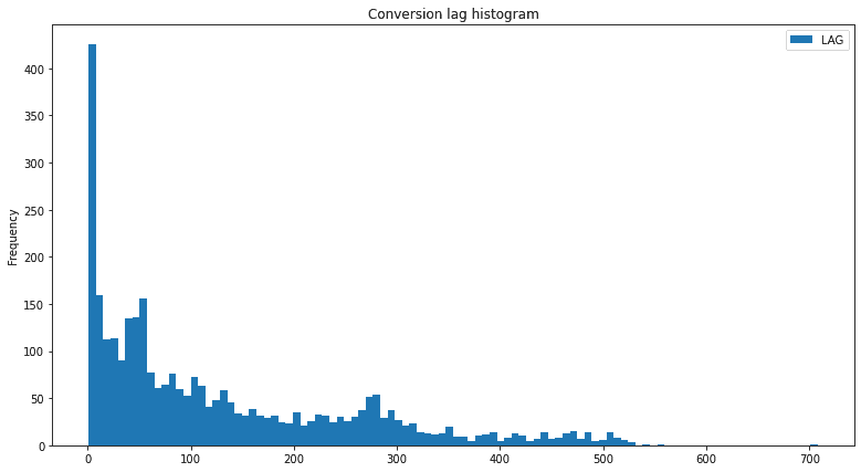
This shows that many users came to the website to request the demo within the first seconds of their visit. Which means they knew about the product. And it shows the imperfection of the tracking. For the web sites, where users log into their accounts, attribution is more precise.
sp_df_cached.select('START_TSTAMP',  "CONVERTED_DATE").sort("START_TSTAMP").to_pandas().plot.scatter(x='START_TSTAMP', y='CONVERTED_DATE', figsize=(15, 10), title="Time gap between first visit and conversion")
<matplotlib.axes._subplots.AxesSubplot at 0x7f6b62bd50d0>
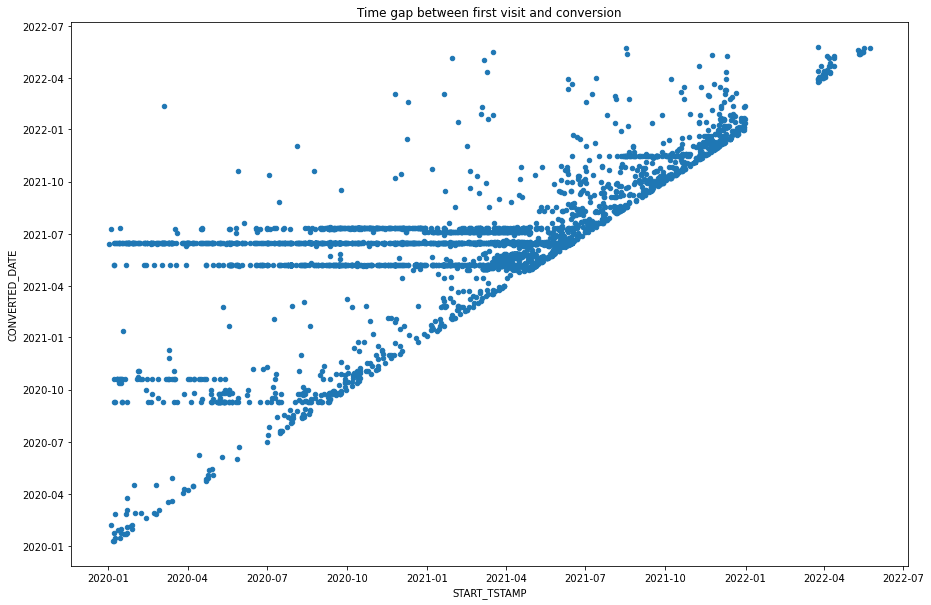
So many customers were waiting for some trigger before conversion around 2020-07 and 2020-10.
For the further investigation of categorical features, we need a helper function to get classes with most variance. For categorical features, a variance threshold has an effect similar to most frequent common features.
from sklearn.preprocessing import OneHotEncoder
from sklearn.feature_selection import VarianceThreshold

def enc_and_select_var(X_:pd.DataFrame, var=0.1) -> pd.DataFrame:
    """
    Encode with one hot encoder and select features over variance threshold
    :param X_: categorical dataframe
    :param var: variance threshold
    :return: transformed dataframe
    """
    oh_enc = OneHotEncoder()
    data = oh_enc.fit_transform(X_)
    ecn_X_ = pd.DataFrame.sparse.from_spmatrix(data, columns=oh_enc.get_feature_names_out())
    thresh = VarianceThreshold(var)
    ecn_best_X_ = thresh.fit_transform(ecn_X_)
    idx_mask = pd.Series(thresh.variances_)
    columns_t = list(pd.Series(ecn_X_.columns)[idx_mask[idx_mask > thresh.threshold].index])
    return pd.DataFrame.sparse.from_spmatrix(ecn_best_X_, columns=columns_t, index = X_.index)
df_2021_07_to_08 = sp_df_cached.where((~is_null(sp_df_cached.CONVERTED_DATE)) & sp_df_cached.CONVERTED_DATE.between('2021-07-01', '2021-07-31')).select(*ref_cols, *mkt_cols, 'START_TSTAMP').to_pandas().astype({
    "START_TSTAMP": "datetime64"
}).set_index('START_TSTAMP')
ecn_best_df_2021_07_to_08_rolling = enc_and_select_var(df_2021_07_to_08).resample("1D").sum().rolling(10).mean()
ecn_best_df_2021_07_to_08_rolling2 = enc_and_select_var(df_2021_07_to_08, 0.05).resample("1D").sum().rolling(10).mean()
ecn_best_df_2021_07_to_08_rolling3 = enc_and_select_var(df_2021_07_to_08, 0.01).resample("1D").sum().rolling(10).mean()
_, axes = plt.subplots(nrows=10, constrained_layout=True, figsize = (13,40))
ecn_best_df_2021_07_to_08_rolling.filter(regex='MKT_.*(?<!None)$', axis=1).plot(kind='line', ax = axes[0], title="Marketing attributes of the initial touch for the users converted on 2021-07 during spike. (Variance 0.1 threshold)")
ecn_best_df_2021_07_to_08_rolling.filter(regex='REFR_.*(?<!None)$', axis=1).plot(kind='line', ax = axes[1], title="Referrer of the initial touch for the users converted on 2021-07 during spike. (Variance 0.1 threshold)")
ecn_best_df_2021_07_to_08_rolling2.filter(regex='MKT_.*(?<!None)$', axis=1).filter(like='MKT_', axis=1).plot(kind='line', ax = axes[2], title="Marketing attributes of the initial touch for the users converted on 2020-07 during spike. (Variance 0.05 threshold)")
ecn_best_df_2021_07_to_08_rolling2.filter(regex='REFR_.*(?<!None)$', axis=1).plot(kind='line', ax = axes[3], title="Referrer of the initial touch for the users converted on 2021-07 during spike. (Variance 0.05 threshold)")
ecn_best_df_2021_07_to_08_rolling3.filter(regex='MKT_SOURCE_.*(?<!None)$', axis=1).plot(kind='area', ax = axes[4], title="Marketing attributes of the initial touch for the users converted on 2021-07 during spike. (Variance 0.01 threshold)")
ecn_best_df_2021_07_to_08_rolling3.filter(regex='MKT_CAMPAIGN_.*(?<!None)$', axis=1).plot(kind='area', ax = axes[5], title="Marketing attributes of the initial touch for the users converted on 2021-07 during spike. (Variance 0.01 threshold)")
ecn_best_df_2021_07_to_08_rolling3.filter(regex='MKT_CONTENT_.*(?<!None)$', axis=1).plot(kind='area', ax = axes[6], title="Marketing attributes of the initial touch for the users converted on 2021-07 during spike. (Variance 0.01 threshold)")
ecn_best_df_2021_07_to_08_rolling3.filter(regex='MKT_SOURCE_.*(?<!None)$', axis=1).plot(kind='area', ax = axes[7], title="Marketing attributes of the initial touch for the users converted on 2021-07 during spike. (Variance 0.01 threshold)")
ecn_best_df_2021_07_to_08_rolling3.filter(regex='REFR_URLHOST_.*(?<!None)$', axis=1).plot(kind='area', ax = axes[8], title="Referrer of the initial touch for the users converted on 2021-07 during spike. (Variance 0.01 threshold)")
ecn_best_df_2021_07_to_08_rolling3.filter(regex='REFR_MEDIUM_.*(?<!None)$', axis=1).plot(kind='area', ax = axes[9], title="Referrer of the initial touch for the users converted on 2021-07 during spike. (Variance 0.01 threshold)")

There are few conclusions that could be made from the conversion spike data
- Most converted visitors came through Google search. (REFR_MEDIUM figure)
- Marketing webinars were successful at attracting visitors that later converted. (MKT_CAMPAIN figure)
- Google Ads was a significant contributor (MKT_SOURCE figure)
- Email campaigns were effective (MKT_SOURCE figure)
A similar approach could be taken to drill down into other features.
Checking landing pages:
from snowflake.snowpark.functions import col
sp_df_cached.where(sp_df_cached.CONVERTED_USER).select('FIRST_PAGE_TITLE').group_by('FIRST_PAGE_TITLE').count().sort(col("COUNT").desc()).show(30)
----------------------------------------------------------------
|"FIRST_PAGE_TITLE"                                  |"COUNT"  |
----------------------------------------------------------------
|Collect_manage_and_operationalize_behavioral_da...  |453      |
|Snowplow_|_The_Data_Collection_Platform_for_Dat...  |326      |
|Treating_data_as_a_product                          |158      |
|White_paper_Introductory_guide_to_data_modeling...  |145      |
|Collect_and_operationalize_behavioral_data_at_s...  |142      |
|Data_modeling_101                                   |102      |
|eBook_Using_data_to_develop_killer_products_|_S...  |96       |
|White_paper_Transform_behavioral_data_into_acti...  |93       |
|Snowplow_|_Introducing_DataOps_into_your_data_m...  |76       |
|Market_Guide_for_Event_Stream_Processing_|_Snow...  |76       |
|Snowplow_|_Explicit_vs_implicit_tracking            |57       |
|Avoid_drowning_in_your_data_lake                    |52       |
|Webinar_The_roadmap_to_data-infomed_customer_jo...  |51       |
|Level_up_your_marketing_attribution_with_the_ad...  |48       |
|The_Future_of_Web_Analytics_A_fireside_chat_wit...  |46       |
|White_paper_A_guide_to_better_data_quality_|_Sn...  |43       |
|Gartner_Report_Introducing_DataOps_into_your_da...  |41       |
|White_paper_How_to_manage_your_data_lake_effect...  |39       |
|Snowplow_|_Data_modeling_mini_series_-_Data_mod...  |38       |
|Snowplow_|_Lessons_learned_from_growing_a_data_...  |37       |
|Snowplow_Webinar_How_Strava_built_a_self-serve_...  |37       |
|Rethinking_web_analytics_for_the_modern_age         |30       |
|Snowplow_webinar_Behavioral_analytics_in_real_time  |28       |
|Snowplow_|_Identity_resolution_in_a_privacy_con...  |25       |
|Snowplow_Webinar_Whats_in_store_for_behavioural...  |23       |
|Snowplow_Webinar_The_new_category_of_the_revers...  |23       |
|Get_started_with_your_Snowplow_Insights_demo_|_...  |21       |
|Webinar_How_to_get_your_data_team_a_seat_at_the...  |21       |
|Map_your_end-to-end_customer_journey_with_behav...  |20       |
|Snowplow_|_People_and_process_in_data_-_A_fires...  |19       |
----------------------------------------------------------------


sp_df_cached.select('FIRST_PAGE_TITLE').group_by('FIRST_PAGE_TITLE').count().sort(col("COUNT").desc()).show(30)
----------------------------------------------------------------
|"FIRST_PAGE_TITLE"                                  |"COUNT"  |
----------------------------------------------------------------
|White_paper_Introductory_guide_to_data_modeling...  |103994   |
|Collect_manage_and_operationalize_behavioral_da...  |98423    |
|Snowplow_|_The_Data_Collection_Platform_for_Dat...  |72360    |
|Treating_data_as_a_product                          |44614    |
|White_paper_Transform_behavioral_data_into_acti...  |17107    |
|Collect_and_operationalize_behavioral_data_at_s...  |16499    |
|Data_modeling_101                                   |14545    |
|The_top_14_open_source_analytics_tools_in_2021_...  |10039    |
|eBook_Using_data_to_develop_killer_products_|_S...  |9762     |
|Snowplow_Analytics_Privacy_Policy_|_Snowplow        |8630     |
|White_paper_A_guide_to_better_data_quality_|_Sn...  |8594     |
|Rethinking_modern_web_analytics                     |6144     |
|Level_up_your_marketing_attribution_with_the_ad...  |5730     |
|Avoid_drowning_in_your_data_lake                    |5497     |
|Work_for_Snowplow_and_join_our_growing_team_|_S...  |4798     |
|Snowplow_Careers_|_Come_And_Be_a_Part_of_Our_Team   |4369     |
|White_paper_How_to_manage_your_data_lake_effect...  |4356     |
|Get_started_with_your_Snowplow_Insights_demo_|_...  |3868     |
|An_introduction_to_event_data_modeling              |3702     |
|Privacy_policy                                      |3635     |
|Three_Ways_to_Derive_Information_From_Event_Str...  |3392     |
|Building_a_model_for_event_data_as_a_graph          |3371     |
|Snowplow_|_Introducing_DataOps_into_your_data_m...  |3313     |
|Snowplow_Insights_|_A_Data_Collection_Platform_...  |2855     |
|Market_Guide_for_Event_Stream_Processing_|_Snow...  |2732     |
|Introducing_SchemaVer_for_semantic_versioning_o...  |2666     |
|A_guide_to_data_team_structures_with_6_examples...  |2664     |
|Snowplow_&_Census_eBook                             |2528     |
|A_guide_to_better_data_quality                      |2354     |
|The_leading_open_source_behavioral_data_managem...  |2326     |
----------------------------------------------------------------
Landing page the converted users look different to the general population. So we could expect a lift in model performance from adding this feature.
Missing values
One common approach to missing values is to extrapolate from the other features with KNN or similar methods. But it would only makes sense, if these features defined in the same row. Snowpark ability to reflect column names comes useful here again.
na_df = sp_df_cached.select([is_null(f).as_(f) for f in sp_df_cached.columns]).to_pandas()
fig = plt.figure()
ax = fig.add_subplot(111)
cax = ax.matshow(na_df.corr(), interpolation='nearest', cmap='coolwarm', aspect='auto', vmin=-1, vmax=1)
fig.colorbar(cax)
xaxis = np.arange(len(df.columns))
ax.tick_params(axis='x', labelrotation=270)
ax.set_xticks(xaxis)
ax.set_yticks(xaxis)
ax.set_xticklabels(df.columns)
ax.set_yticklabels(df.columns)
ax.set_xticklabels([''] + df.columns)
ax.set_yticklabels([''] + df.columns)
ax.set_title("N/A correlation matrix", y=1.31)
fig.set_size_inches(12, 10)
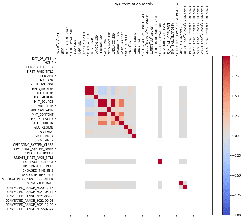
It would be wrong to fill in marketing source, because missing values there are meaningful. BR_LANG and GEO_* could be interpolated from other features as they show small correlation.
from snowflake.snowpark.functions import datediff


_, axes = plt.subplots(2, 3, figsize=(14, 14))

data_converted = sp_df_cached.where(sp_df_cached.CONVERTED_USER).select(
 *engagement_cols
).to_pandas()

data = sp_df_cached.select(
    *engagement_cols
).to_pandas()

data.VERTICAL_PERCENTAGE_SCROLLED.plot(bins=100, kind='hist', title = "VERTICAL_PERCENTAGE_SCROLLED for all users", ax=axes[0][0])
data.ENGAGED_TIME_IN_S.plot(bins=100, kind='hist', logy=True, title = "ENGAGED_TIME_IN_S for all users", ax=axes[0][1])
data.ABSOLUTE_TIME_IN_S.plot(bins=100, kind='hist', logy=True, title = "ABSOLUTE_TIME_IN_S for all users", ax=axes[0][2])
data_converted.VERTICAL_PERCENTAGE_SCROLLED.plot(bins=100, kind='hist', title = "VERTICAL_PERCENTAGE_SCROLLED for converted users", ax=axes[1][0])
data_converted.ENGAGED_TIME_IN_S.plot(bins=100, kind='hist', logy=True, title = "ENGAGED_TIME_IN_S for converted users", ax=axes[1][1])
data_converted.ABSOLUTE_TIME_IN_S.plot(bins=100, kind='hist',logy=True,  title = "ABSOLUTE_TIME_IN_S for converted users", ax=axes[1][2])
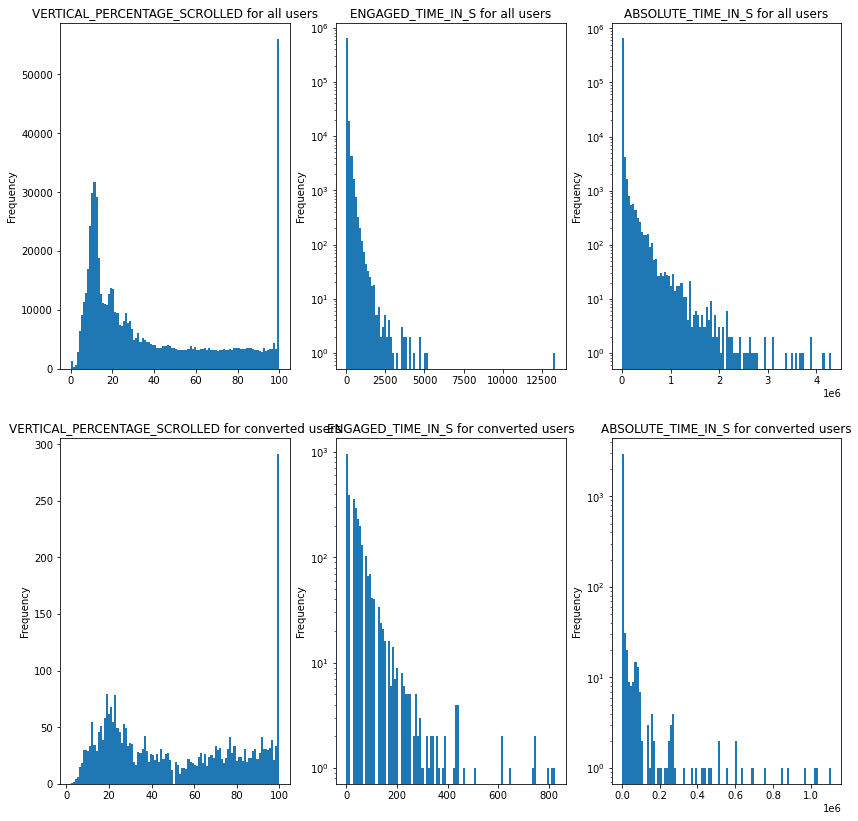
Continues features have logarithmic distribution. For linear models they need to be scaled.
References
[1] Shao, Xuhui, and Lexin Li. “Data-driven multi-touch attribution models.” Proceedings of the 17th ACM SIGKDD international conference on Knowledge discovery and data mining. 2011.
[2] R. Berman, “Beyond the Last Touch: Attribution in Online Advertising,” Marketing Science, vol. 37, no. 5, pp. 771–792, Sep. 2018, doi: 10.1287/mksc.2018.1104.
[3] https://developers.google.com/ads-data-hub/reference/table-schemas/vendors#google-ads-campaign
[4] Wright, Raymond E. “Logistic regression.” (1995).
[5] Ke, G., Meng, Q., Finley, T., Wang, T., Chen, W., Ma, W., Ye, Q. and Liu, T.Y., 2017. Lightgbm: A highly efficient gradient boosting decision tree. Advances in neural information processing systems, 30.
[6] https://shap-lrjball.readthedocs.io/en/latest/index.html
[7] https://snowplow.github.io/dbt-snowplow-web/#!/model/model.snowplow_web.snowplow_web_users
[8] https://docs.snowplow.io/docs/enriching-your-data/available-enrichments/yauaa-enrichment/
[9] https://docs.snowplow.io/docs/enriching-your-data/available-enrichments/ua-parser-enrichment/
[10] https://docs.snowplow.io/docs/enriching-your-data/available-enrichments/cookie-extractor-enrichment/
[11] https://docs.snowplow.io/docs/enriching-your-data/available-enrichments/ip-lookup-enrichment/
[12] https://docs.snowplow.io/docs/enriching-your-data/available-enrichments/iab-enrichment/
[13] https://snowplow.github.io/dbt-snowplow-web/#!/model/model.snowplow_web.snowplow_web_page_views

