Building a “Propensity to Convert” machine learning model with Snowpark and Snowplow web tracking - Part 2
The following guide is a continuation of part 1 in our series on how to build a propensity-to-convert machine learning model with Snowplow and Snowplow. In part 2, we’ll be looking at folding, modeling, scoring, and loading into Snowflake.
Folding
Consider an example where a user came to our website last year but converted yesterday. If we were to train the model a month ago, it would consider this user a negative class, but today’s model will consider the same user converted.
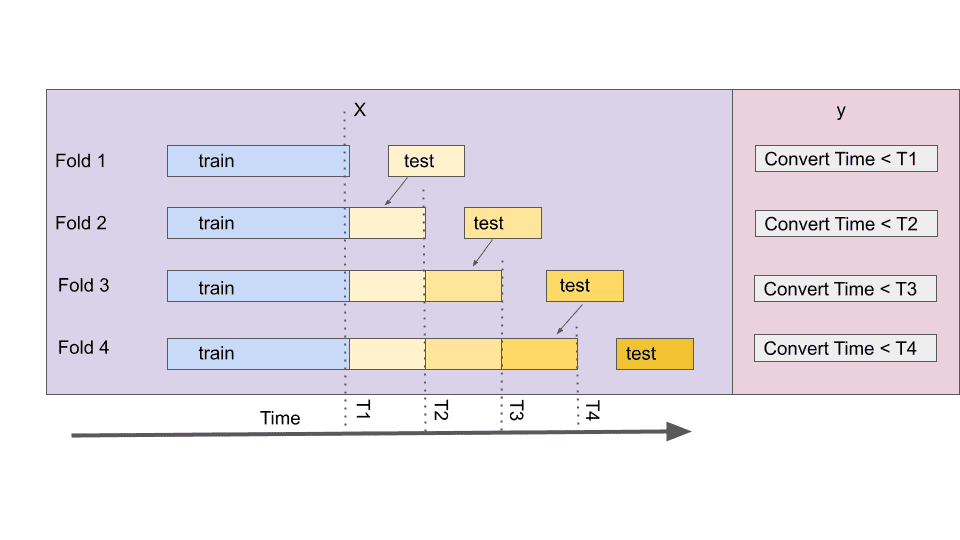
This quality prevents incremental model training when the same features could change class between folds. Moreover, it also has consequences for GridSearch, which cannot accept indices for X and y separately. So folds would have to be constructed manually.
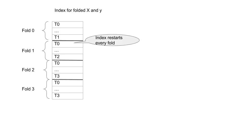
df.reset_index(inplace=True)
folds = []
fold_idxs= []

y_folded = pd.Series(dtype=object)
X_folded = pd.DataFrame()
for name, cutoff in zip(step_names, step_dates):
    X_train = df.loc[df.START_TSTAMP < cutoff].copy()
    y_train = X_train[name]
    X_test =  df.loc[(df.START_TSTAMP > cutoff) & (df.START_TSTAMP <= cutoff + step_duration )]
    y_test = X_test[name]
    train_idx_start = len(y_folded)
    len_train = len(y_train)
    len_test = len(y_test)
    y_folded = pd.concat([y_folded, y_train, y_test], ignore_index=True)
    X_folded = pd.concat([X_folded, X_train, X_test], ignore_index=True)
    fold_idxs.append(
        (pd.RangeIndex(train_idx_start ,
                      train_idx_start + len_train),
        pd.RangeIndex(train_idx_start + len_train,
                      train_idx_start + len_train + len_test)
    ))
    # time series have a rounding issues with selection by index.
    assert X_train.shape == X_train.loc[X_train.index].shape
    folds.append( (X_train, y_train, X_test, y_test))
Since we will be passing indexes into the GridSearch it is critical to verify their consistency. assert_array_almost_equal is required for the float comparison.
import numpy as np
import sys

np.set_printoptions(threshold=sys.maxsize, linewidth=sys.maxsize)

for fold, fold_idx, name in zip(folds, fold_idxs, step_names):
    X_train, y_train, X_test, y_test = fold
    train_idx, test_idx = fold_idx
    np.testing.assert_array_equal(X_train[discrete_col ], X_folded.loc[train_idx, discrete_col], verbose=True)
    np.testing.assert_array_almost_equal(X_train[continues_col ], X_folded.loc[train_idx, continues_col ])
    np.testing.assert_array_equal(X_test[discrete_col ], X_folded.loc[test_idx, discrete_col], verbose=True)
    np.testing.assert_array_almost_equal(X_test[continues_col ], X_folded.loc[test_idx, continues_col ])
    np.testing.assert_array_equal(y_train,  y_folded[train_idx], verbose=True)
    np.testing.assert_array_equal(y_test,  y_folded[test_idx], verbose=True)

print("Fold validation complete.")
Fold validation complete.
Model selection
Finding the accurate parameters for the model is done with the GridSearchCV. Nevertheless, before automatic selection can be used, initial pipeline for the model must be defined.
Imputation
Most pipelines start with filling missing values. This process is called imputation, and there are three popular methods of doing it:
- Replacing a missing value with a constant value. This works well for categorical columns.
- Using the mean of the series. Suitable for continuous columns, such as engaged time or scroll.
- Column value from the other columns. This is the area of active research. The most established solution is K-nearest neighbour (KNN).
- Train another model to fill in the missing values.
For the baseline model, it is best to start with simple imputation – constant and mean value. KNN or other more advanced methods.In this pipeline, constant replacement is used for categorical values and mean for continuous ones. Boolean column SPIDER_OR_ROBOT is assumed to be false.
Encoding and Transformation
The majority of classifiers/regressors do not allow categorical features unencoded. So they must be turned into a numeric representation. The OneHotEncoder performs the most straightforward transformation, creating a column per each category.
Linear models could deal with scaling features or weird distributions. However, there is a hidden problem. Feature importance (linear model coefficients) is used in marketing attribution. Consider Google Ads encoded as 1 and Google Search encoded as 2. The linear model will have to scale Ads by a factor of 2, so a naive marketing attribution model trained on random data will show that Ads are twice as important.
A prefered way of evaluating feature importance is with SHAP, which will fix this issue for linear models.
For text fields, like item description or comment content, nltk provides guidance and a rich set of functionality. By default, Snowplow does not collect any free text fields. Images are rare in behavioral data, and there is a vast body of research on their classification. Both text and image classification perform much better with the transformer neural networks. While categorical data does well with decision trees. One solution could be to train separate models for each text/image field and integrate model outputs as an input feature for the behavioral model.In this pipeline, categorical features are encoded with OneHotEncoder and continuous ones transformed with StandardScaler.
Selection of best features
Often model performance improves when the number of features is reduced, also known as the dimensionality curse. The linear model assumes feature independence. Moreover, marketing features are rarely independent; e.g. marketing campaigns applied to specific regions. Regularization solves this requirement but only for the linear relationship, which rarely exists.
Another reason to reduce the number of features is interpretability. SHAP does not scale well with more features.
Having many rare features could cause overwriting. For example, if a single user found our website in the Urdu language and later converted, the model could learn that and penalize all English users, even though they constitute 99% of conversions. This issue could be solved by model tuning, but it is better not to have this problem.
A reasonable starting point for the feature selection is the Variance threshold, which excludes features that do not change much. The default value of threshold 0 will exclude the constant columns. Consider trying it with 0.01 or 0.001.
Features could be selected as feature importance of different models, mutual information test, correlation or chi2 test. See this excellent guide from sklearn for more on this.In this article, each group of features uses the chi2 test. This is done per group to guarantee that the entire feature group is excluded from the model. The next step is VarianceThreshold(0) to exclude constant features.
Class Balancing
The imbalance ratio 0.0046 of converted against non-converted users is the defining property of this project. That degree of imbalance is a difficult challenge because there is not enough data to represent the positive cases. If imbalance is not addressed, the model would predict 0 (not converted) for every sample. Which would leave the excellent accuracy of ~99.5%, same as the ratio of negative class. The considered solutions:
- Class weight: Some classifiers allow to pass class weights as part of tuning. Which integrates with loss function calculation.
- Under sampling: Each class selects the same number of rows. This example model will lose 99% of the data – 0.5% is for positive class – 0.5% for negative class and 99% of negative class discarded.
- Over sampling: Generate synthetic data from the positive classes available. For example by using KNN or inserting Gaussian noise for continuous features.
Both class weights and under sampling could suffer from overfitting. With enough parameters, the model encodes all 3000 positive samples in the model’s coefficients.Imbalanced learn is an excellent library that implements over/under sampling methods. Note that ADASYN is much slower than SMOTE, so it might be a good idea to start with later.
Classifier
A final step of the pipeline is a classification algorithm that would take our preprocessed features and return the prediction, class probability and feature importance. Logistic regression is the most well-known model. It is easy to reason with just a graduate knowledge of statistics, making it a perfect candidate for the baseline.
Boosting trees perform better than neural networks on categorical data sets, such as this one. Another great property is their ability to work with noisy data, LightGBM could do all preprocessing internally, but this isn’t used in this article. The most popular ones are XGBoost, LightGBM and CatBoost, each with different strengths The overall winner for accuracy is CatBoost,which is also the newest.
In this article LightGBM is used because the author was more familiar with it. Respectably, all are mature libraries for big corporations IBM, Microsoft and Yandex, so do not expect drastic performance gains from swapping one for the other.
from imblearn.over_sampling import SMOTE
from imblearn.under_sampling import  RandomUnderSampler
import sklearn
from sklearn.compose import ColumnTransformer
from sklearn.impute import SimpleImputer
from sklearn.linear_model import LogisticRegression
from sklearn.preprocessing import  OneHotEncoder, StandardScaler
from imblearn.pipeline import make_pipeline, Pipeline
from sklearn.feature_selection import  VarianceThreshold, SelectKBest
import lightgbm as lgb
from sklearn import set_config
from sklearn.utils import estimator_html_repr
from silent_lgbm import SilentLGBMClassifier

# this will make jupiter output pretty interactive diagrams
set_config(display="diagram")

def make_category_pipe(k_best=10):
    return sklearn.pipeline.make_pipeline(
        SimpleImputer(strategy='constant'),
        OneHotEncoder(handle_unknown='ignore'),
        SelectKBest(sklearn.feature_selection.chi2, k=k_best)
    )


# robot and spider enrichment pipe
robot_pope = sklearn.pipeline.make_pipeline(SimpleImputer(strategy='constant', fill_value=False, missing_values=None),
                           OneHotEncoder(handle_unknown='ignore'))

# engagement metrics pipe
engaged_pipe = sklearn.pipeline.make_pipeline(SimpleImputer(strategy='mean'), StandardScaler())

pre_steps = [ColumnTransformer(
    [
        ("REF", make_category_pipe(20), ref_cols),
        ("MKT", make_category_pipe(20), mkt_cols),
        ("GEO", make_category_pipe(20), geo_cols),
        ("DEV", make_category_pipe(20), dev_cols),
        ("ROBOT", robot_pope, robot_cols),
        ("TITLE", make_category_pipe(40), url_cols),
        ("CALENDAR", make_category_pipe(24 + 7), calendar_cols),
        ("ENGAGED", engaged_pipe, engagement_cols)
    ]
    , remainder='drop'),
    VarianceThreshold(0),
    SMOTE()
]

# Some of the paramerter were already found with GridSearch. Normally start with defaults - LogisticRegression().
# class weight are discussed later.
clf_l = LogisticRegression(solver='saga', penalty ='elasticnet', l1_ratio=0.2,
                                                   class_weight= {True: 2, False: 1}
                                              )


# LightGBM gets chatty about iterations, categorical features and this is simple wrapper to get discard user warning.
# It needs to be in separate file, so joblib could serialize it correctly, which would be required for loading this model into snowflake
clf =  SilentLGBMClassifier(importance_type='gain', objective='binary', force_col_wise='True', learning_rate=0.01, scale_pos_weight=2)

pipe_lgbm = Pipeline(list(zip(["preprocessing", "selector", "sampler", "clf"], [*pre_steps, clf] )))
pipe_lin = Pipeline(list(zip(["preprocessing", "selector", "sampler", "clf"], [*pre_steps, clf_l] )))

## Saves html iteractive diagram of the pipeline. We can't embed html into the blog. So it is shown as picture.
with open('estimator.html', 'w') as f:
    f.write(estimator_html_repr(pipe_lgbm))

pipe_lgbm
Pipeline(steps=[('preprocessing',
                 ColumnTransformer(transformers=[('REF',
                                                  Pipeline(steps=[('simpleimputer',
                                                                   SimpleImputer(strategy='constant')),
                                                                  ('onehotencoder',
                                                                   OneHotEncoder(handle_unknown='ignore')),
                                                                  ('selectkbest',
                                                                   SelectKBest(k=20,
                                                                               score_func=<function chi2 at 0x7f2d22357c10>))]),
                                                  ['REFR_URLHOST',
                                                   'REFR_MEDIUM', 'REFR_TERM',
                                                   'REFR_ANY']),
                                                 ('MKT',
                                                  Pipeline(ste...
                                                  Pipeline(steps=[('simpleimputer',
                                                                   SimpleImputer()),
                                                                  ('standardscaler',
                                                                   StandardScaler())]),
                                                  ['ENGAGED_TIME_IN_S',
                                                   'ABSOLUTE_TIME_IN_S',
                                                   'VERTICAL_PERCENTAGE_SCROLLED'])])),
                ('selector', VarianceThreshold(threshold=0)),
                ('sampler', SMOTE()),
                ('clf',
                 SilentLGBMClassifier(force_col_wise='True',
                                      importance_type='gain',
                                      learning_rate=0.01, objective='binary',
                                      scale_pos_weight=2))])
Scoring
Before fitting model hyperparameters, it is essential to establish what model property is being maximized. Read about machine learning scoring (accuracy, F1, precision and recall) here. Accuracy would not work for this data due to class imbalance. A common approach to avoid this issue is the F1 score – a harmonic mean of precision and recall.
Identifying conversions (true positive) is more important than misclassifying negatives (false positives). Because F1 assigns the same weight to both precision and recall, it needs to be generalized to F Beta. That allows us to wight recall against precision.F2 (beta equals 2) is used for this task – recall is twice as important as precision. The value of beta should be tuned to a business case.
Grid Search
With all the preparation done so far, running GridSearch is easy. Finding the right hyperparameters for the model is computationally expensive. Grid search will iterate over all combinations in parameter space. Which means O(n!) complexity. For example, if 4 parameters are varied and our training set is split 6 ways, GridSearch will train our model 4! * 6 = 24 * 6 = 144 times.
sklearn has an experimental HalvingGridSearchCV version, which will reduce the number of candidates by a factor of 3 (tunable default) every folding iteration.
Please note that this is an oversimplified explanation. The actual algorithm is more complex (it is not always 3). Please read the user guide for full detail.HalvingGridSearchCV is much faster because it runs fewer training iterations, allowing it to be a bit more liberal with search parameters space. However, it is still important to consider training times when choosing parameters.
Linear Model
The logistic regression model is chosen as the baseline as the simplest classification model available. Saga solver is sufficiently fast for this and does not require additional tuning.
from  sklearn.metrics import make_scorer, fbeta_score

scorer = make_scorer(fbeta_score, beta=2, pos_label=True)
from sklearn.experimental import enable_halving_search_cv
from sklearn.model_selection import HalvingGridSearchCV

cv_params_lin = [{
    "preprocessing__REF__selectkbest__k":  [10],
    "preprocessing__MKT__selectkbest__k":  [10],
    "preprocessing__GEO__selectkbest__k":  [10],
    "preprocessing__DEV__selectkbest__k":  [10],
    "preprocessing__TITLE__selectkbest__k":  [10],
    "preprocessing__CALENDAR__selectkbest__k":  [10],
    'sampler': [SMOTE(), RandomUnderSampler()],
    "clf__l1_ratio": [ 0, 0.25, 0.5 , 0.75, 1],
    "clf__C": [  0.05, 0.25, 0.5, 1 , 2  ]
    },
    {
    "preprocessing__REF__selectkbest__k":  [50],
    "preprocessing__MKT__selectkbest__k":  [50],
    "preprocessing__GEO__selectkbest__k":  [50],
    "preprocessing__DEV__selectkbest__k":  [50],
    "preprocessing__TITLE__selectkbest__k":  [50],
    "preprocessing__CALENDAR__selectkbest__k":  ['all'],
    'sampler': [SMOTE(), RandomUnderSampler()],
    "clf__l1_ratio": [ 0, 0.25, 0.5 , 0.75, 1],
    "clf__C": [ 0.05, 0.25, 0.5, 1 , 2 ]
    },{
    "preprocessing__REF__selectkbest__k":  [100],
    "preprocessing__MKT__selectkbest__k":  [100],
    "preprocessing__GEO__selectkbest__k":  [100],
    "preprocessing__DEV__selectkbest__k":  [100],
    "preprocessing__TITLE__selectkbest__k":  [100],
    "preprocessing__CALENDAR__selectkbest__k":  ['all'],
    'sampler': [SMOTE(), RandomUnderSampler()],
    "clf__l1_ratio": [ 0, 0.25, 0.5 , 0.75, 1],
    "clf__C": [  0.05, 0.25, 0.5, 1 , 2  ]
    }
]

gs_l = HalvingGridSearchCV(pipe_lin, cv_params_lin, cv=fold_idxs, verbose=1, n_jobs=-1, scoring=scorer)
gs_l.fit(X_folded, y_folded)

import pickle as pkl
with open("gs_lin.pckl", "wb") as file:
    pkl.dump(gs_l, file)
n_iterations: 5
n_required_iterations: 5
 n_possible_iterations: 5
min_resources_: 36271
max_resources_: 2937980
 aggressive_elimination: False factor: 3
 ----------
iter: 0
n_candidates: 150
 n_resources: 36271
Fitting 6 folds for each of 150 candidates, totalling 900 fits
 ---------
iter: 2
 n_candidates: 17
 n_resources: 326439
Fitting 6 folds for each of 17 candidates, totalling 102 fits
 ----------
iter: 3 n_candidates: 6
n_resources: 979317
Fitting 6 folds for each of 6 candidates, totalling 36 fits
----------
iter: 4
n_candidates: 2
n_resources: 2937951
Fitting 6 folds for each of 2 candidates, totalling 12 fits
Helper functions are defined to inspect the results further
- Plot confusion matrixes and F2 scores for each fold.
- Get real column names, required because OneHotEncoder, SelectKBest and VarianceThreshhold mangle original columns.
- Display the GridSearch results: Search grids are often multidimensional, and it is impossible to draw 4 dimensions; even 3 dimensions could be challenging with few points. Function outputs a series of heatmaps which show scores for each combination of two parameters, with other parameters set to optimal values.
Hyper tuning takes a long time to run ~4 hours of xlarge AWS instance. Th results are staged into the filesystem, so the GridSearch results could be loaded and analyzed later.
Two final candidate parameters are shown to illustrate the shape of the data. In practice, mean_fit_time should be considered alongside the mean_test_score, as it impacts research speed. It makes sense to sacrifice some accuracy for performance.
import pickle as pkl
with open("gs_lin.pckl", "rb") as file:
    gs_l = pkl.load(file)

gs_results = pd.DataFrame.from_dict(gs_l.cv_results_)
gs_results[gs_results.iter == 4].sort_values('mean_test_score', ascending=False)
     iter  n_resources  mean_fit_time  std_fit_time  mean_score_time  \
223     4      2937951     271.053132    129.039554         1.205354
224     4      2937951     256.987730    113.300479         1.156112
We could inspect the best parameter combination and what F2 scores were.
gs_l.best_params_
{'clf__C': 0.5,
 'clf__l1_ratio': 0.25,
 'preprocessing__CALENDAR__selectkbest__k': 'all',
 'preprocessing__DEV__selectkbest__k': 50,
 'preprocessing__GEO__selectkbest__k': 50,
 'preprocessing__MKT__selectkbest__k': 50,
 'preprocessing__REF__selectkbest__k': 50,
 'preprocessing__TITLE__selectkbest__k': 50,
 'sampler': SMOTE()}
gs_l.best_score_
0.03930983408691514
Plotting results of GridSearch is challenging when parameter space has more than two dimensions. So each pair of parameters were projected onto the combination of the remainder of the best parameters.
HalvingGridSearch is aggressive in eliminating parameter combinations, so many parameters in that project are set to 0.
_, axes =  plt.subplots(4, 4, figsize=(13, 13), sharey='row', sharex='col', constrained_layout=True)

# only inspecting `preprocessing__TITLE__selectkbest__k` because other preprocessing__* change together with it
for i, x_col in enumerate(["clf__C", "clf__l1_ratio", "sampler", "preprocessing__TITLE__selectkbest__k" ]):
    for j, y_col in enumerate(["clf__C", "clf__l1_ratio", "sampler", "preprocessing__TITLE__selectkbest__k"]):
        if i <=j:
            axes[i,j].set_visible(False)
            continue
        make_heatmap(axes[i][j], gs_l, y_col, x_col, show_x=i==3, show_y=j==0, what_to_how='mean_test_score')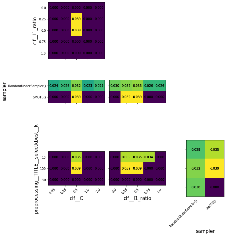
The following figures inspect the results and scores for each fold. During training, we got warnings about The max_iter was reached which means the coef_ did not converge, which indicates that the linear model is not a good fit for this problem or the model needs further tuning of the stopping criteria.
plot_conf_matrixes(pipe_lin.set_params(**gs_l.best_params_))
SHAP valuation of the linear model. Note that blue and red are gradients, which is a property of a linear model, where features could only have positive or negative impact. In non-linear models the same features and value could be both positive and negative, so this plot won’t be uniform.
import shap
rng = np.random.default_rng()
pipe_lin.set_params(**gs_l.best_params_)
column_pipe = Pipeline(pipe_lin.steps[:-1])
X_train,y_train,  X_test, y_test = folds[-1]
Xt_train, yt_train = column_pipe.fit_resample(X_train, y_train)
Xt_test = Pipeline(column_pipe.steps[:-1]).transform(X_test)
all_cols, cat_cols = get_column_names(column_pipe)
clf_l = pipe_lin.steps[-1][1]
clf_l.fit(Xt_train, yt_train)
arXt = pd.DataFrame(rng.choice(Xt_train.toarray(), 200, replace=False), columns = all_cols)
explainer = shap.explainers.Linear(clf_l,shap.maskers.Independent(Xt_train, max_samples=200))
shap_values = explainer(arXt)
shap.plots.beeswarm(shap_values, show=False)
fig = plt.gcf()
fig.savefig("shap_lin.png", dpi=400, bbox_inches='tight')
plt.show()
The max_iter was reached which means the coef_ did not converge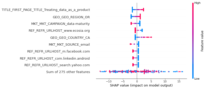
LightGBM model
LightGLightGBM does not necessarily require any preprocessing pipeline steps. Categorical encoding and normalization are part of the library. It uses advanced encoders for categorical features that have few values. Normalization is not required at all for tree boosting algorithms. Several hyperparameters control the selection of input features – the most direct one is min_child_samples. So SelectKBest is also not necessary.
However, SHAP will not work with a massive number of input features, and it cannot do autoencoding. So to make our model explainable, we sacrifice a little bit of accuracy by integrating our classifier into the sklearn pipeline.
from sklearn.experimental import enable_halving_search_cv
from sklearn.model_selection import GridSearchCV, HalvingGridSearchCV

cv_params = [{
    "clf__n_estimators": [10, 25, 50, 100],
    "clf__min_child_samples": [10, 25, 50, 100],
    "clf__num_leaves":[24, 32, 64],
}]

pipe_lgbm.set_params(**{
    "preprocessing__REF__selectkbest__k":  100,
    "preprocessing__MKT__selectkbest__k":  100,
    "preprocessing__GEO__selectkbest__k":  100,
    "preprocessing__DEV__selectkbest__k":  100,
    "preprocessing__TITLE__selectkbest__k":  100,
    "preprocessing__CALENDAR__selectkbest__k":  'all',
    'sampler': SMOTE()
})


gs = HalvingGridSearchCV(pipe_lgbm, cv_params,cv=fold_idxs, verbose=1,  n_jobs=-1, scoring=scorer)
gs.fit(X_folded, y_folded)

import pickle as pkl
with open("gs_lgbm.pckl", "wb") as file:
    pkl.dump(gs, file)
n_iterations: 4
n_required_iterations: 4
n_possible_iterations: 4
min_resources_: 109371
max_resources_: 2953017
aggressive_elimination: False
factor: 3
----------
iter: 0
n_candidates: 48
n_resources: 109371
Fitting 6 folds for each of 48 candidates, totalling 288 fits
----------
iter: 2
n_candidates: 6
n_resources: 984339
Fitting 6 folds for each of 6 candidates, totalling 36 fits
----------
iter: 3
n_candidates: 2
n_resources: 2953017
Fitting 6 folds for each of 2 candidates, totalling 12 fits
import pickle as pkl
with open("gs_lgbm.pckl", "rb") as file:
    gs_lgbm = pkl.load(file)

gs_results = pd.DataFrame.from_dict(gs_lgbm.cv_results_)
gs_results[gs_results.iter == 3].sort_values('mean_test_score', ascending=False)
    iter  n_resources  mean_fit_time  std_fit_time  mean_score_time  \
71     3      2953017      45.311950     14.418792         1.555733
70     3      2953017      44.850752     18.835954         1.854426

 _, axes =  plt.subplots(3, 3, figsize=(13, 13), sharey='row', sharex='col', constrained_layout=True)
for i, x_col in enumerate(["clf__n_estimators", "clf__min_child_samples", "clf__num_leaves"]):
    for j, y_col in enumerate(["clf__n_estimators", "clf__min_child_samples", "clf__num_leaves"]):
        if i<=j:
            axes[i,j].set_visible(False)
            continue
        make_heatmap(axes[i][j], gs_lgbm, y_col, x_col, show_x=i==2, show_y=j==0, what_to_how='mean_test_score')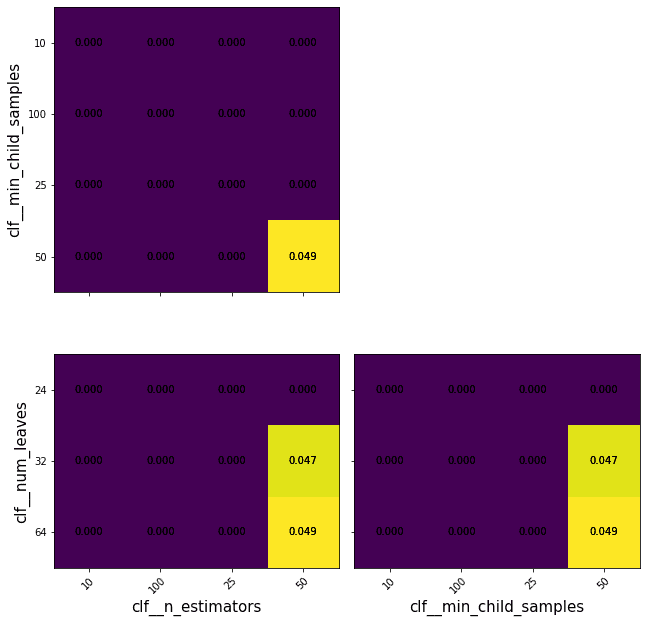
gs_lgbm.best_params_
{'clf__min_child_samples': 100,
 'clf__n_estimators': 100,
 'clf__num_leaves': 64}
gs_lgbm.best_score_
0.04943520760104766
Score is about 25% better than of the baseline linear model.
gs_lgbm.best_score_/ gs_l.best_score_
1.2575786377460927
import shap
import copy

pipe_lgbm.set_params(**gs_lgbm.best_params_)

rng = np.random.default_rng()
column_pipe = Pipeline(pipe_lin.steps[:-1])
X_train,y_train,  X_test, y_test = folds[-1]
Xt_train, yt_train = column_pipe.fit_resample(X_train, y_train)
Xt_test = Pipeline(column_pipe.steps[:-1]).transform(X_test)
all_cols, cat_cols = get_column_names(column_pipe)
clf_g = pipe_lgbm.steps[-1][1]
clf_g.fit(Xt_train, yt_train)
explainer = shap.TreeExplainer(clf_g)
arXt = pd.DataFrame(rng.choice(Xt_train.toarray(), 2000, replace=False), columns = all_cols)
shap_values1 = explainer(arXt)
shap_values2 = copy.deepcopy(shap_values1)
shap_values2.values = shap_values2.values[:,:,1]
shap_values2.base_values = shap_values2.base_values[:,1]
shap.plots.beeswarm(shap_values2)
fig = plt.gcf()
fig.savefig("shap_lgbm.png", dpi=400, bbox_inches='tight')
plt.show()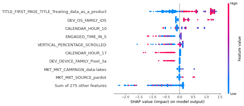
The order of most important features had changed. VERTICAL_PERCANTAGE_SCROLLED moves to the top 5 from the bottom 275, indicating non-linear dependency between this and other features. The move could be explained by the fact that phones need to scroll more than desktops due to the screen size.
plot_conf_matrixes(pipe_lgbm.set_params(**gs_lgbm.best_params_))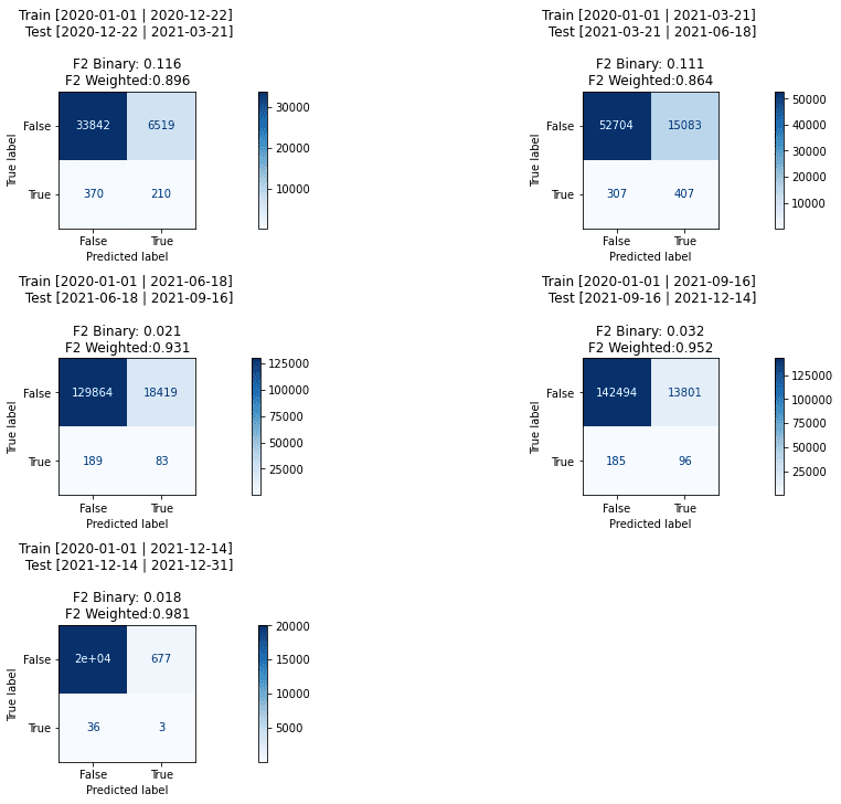
It is interesting to consider how much the engagement metric contributes to the overall accuracy. It turned out to be about 30%.
pipe_lgbm.set_params(**{
    "preprocessing__ENGAGED":  'drop',
})
plot_conf_matrixes(pipe_lgbm.set_params(**gs_lgbm.best_params_))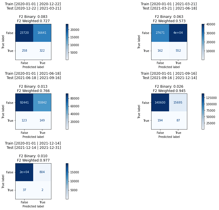
Pipeline(steps=[('preprocessing',
                 ColumnTransformer(transformers=[('REF',
                                                  Pipeline(steps=[('simpleimputer',
                                                                   SimpleImputer(strategy='constant')),
                                                                  ('onehotencoder',
                                                                   OneHotEncoder(handle_unknown='ignore')),
                                                                  ('selectkbest',
                                                                   SelectKBest(k=20,
                                                                               score_func=<function chi2 at 0x7f2d22357c10>))]),
                                                  ['REFR_URLHOST',
                                                   'REFR_MEDIUM', 'REFR_TERM',
                                                   'REFR_ANY']),
                                                 ('MKT',
                                                  Pipeline(ste...
                                                  ['DAY_OF_WEEK', 'HOUR']),
                                                 ('ENGAGED', 'drop',
                                                  ['ENGAGED_TIME_IN_S',
                                                   'ABSOLUTE_TIME_IN_S',
                                                   'VERTICAL_PERCENTAGE_SCROLLED'])])),
                ('selector', VarianceThreshold(threshold=0)),
                ('sampler', SMOTE()),
                ('clf',
                 SilentLGBMClassifier(force_col_wise='True',
                                      importance_type='gain',
                                      learning_rate=0.01, min_child_samples=100,
                                      num_leaves=64, objective='binary',
                                      scale_pos_weight=2))])
Loading the model to Snowflake
Models could be served from Snowflake as a user defined function (UDF).
At the moment snowpark does not support imbalanced-learn, so the pipeline should be stripped of SMOTE and assembled as sklearn pipeline.
from joblib import dump
from sklearn.pipeline import Pipeline

def un_imbalance(p):
    new_steps = []
    if isinstance(p, imblearn.pipeline.Pipeline):
        for step in p.steps:
            if isinstance(step[1], imblearn.pipeline.Pipeline):
                new_steps.append((step[0], un_imbalance(step[1])))
            elif isinstance(step[1], imblearn.over_sampling.SMOTE):
                continue
            else:
                new_steps.append(step)
        return Pipeline(steps=new_steps)

pipe.set_params(**gs.best_params_)
pipe.fit(X, y)

dump(un_imbalance(pipe), 'estimator.joblib')
Model loading must be cached, otherwise performance would make it unusable as it will load on every call.
from snowflake.snowpark.functions import udf
from snowflake.snowpark.types import PandasSeries, PandasDataFrame, IntegerType
from snowflake.snowpark import Session
import cachetools

with open("pavel-snowflake-dev.properties") as file:
    props = dict([l.rstrip().split(" = ", 2) for l in file.readlines() if " = " in l])

session = Session.builder.configs(props).create()
session.add_import("@ANALYTICS_DEV_DB.ML_DEMO.MODEL_STAGE/estimator.joblib")
session.add_import("@ANALYTICS_DEV_DB.ML_DEMO.MODEL_STAGE/silent_lgbm.py")


@cachetools.cached(cache={})
def read_model(filename):
    import sys
    import os
    from joblib import load
    from silent_lgbm import SilentLGBMClassifier
    import_dir = sys._xoptions.get("snowflake_import_directory")
    if import_dir:
        return load(os.path.join(import_dir, filename))

@udf(packages=["numpy", "pandas", "scikit-learn", "cachetools", "lightgbm"], session=session,
     is_permanent=True,
     stage_location='@ANALYTICS_DEV_DB.ML_DEMO.MODEL_STAGE', name='predict',
     imports=["estimator.joblib", "silent_lgbm.py"], replace=True)
def predict(
        REFR_URLHOST: str,
        REFR_MEDIUM: str,
        REFR_TERM: str,
        MKT_MEDIUM: str,
        MKT_SOURCE: str,
        MKT_TERM: str,
        MKT_CAMPAIGN: str,
        MKT_CONTENT: str,
        MKT_NETWORK: str,
        GEO_COUNTRY: str,
        GEO_REGION: str,
        BR_LANG: str,
        DEVICE_FAMILY: str,
        OS_FAMILY: str,
        OPERATING_SYSTEM_CLASS: str,
        OPERATING_SYSTEM_NAME: str,
        SPIDER_OR_ROBOT: str,
        FIRST_PAGE_TITLE: str,
        URL: str,
        HOUR: str,
        DAY_OF_WEEK: str,
        ENGAGED_TIME_IN_S: float,
        ABSOLUTE_TIME_IN_S: float,
        VERTICAL_PERCENTAGE_SCROLLED: float) -> float:
    df0 = pd.DataFrame([[
        REFR_URLHOST,
        REFR_MEDIUM,
        REFR_TERM,
        not not ( REFR_URLHOST or REFR_MEDIUM or REFR_TERM),
        MKT_MEDIUM,
        MKT_SOURCE,
        MKT_TERM,
        MKT_CAMPAIGN,
        MKT_CONTENT,
        MKT_NETWORK,
        not not ( MKT_MEDIUM or  MKT_SOURCE or  MKT_TERM or  MKT_CAMPAIGN or  MKT_CONTENT or MKT_NETWORK),
        GEO_COUNTRY,
        GEO_REGION,
        BR_LANG,
        DEVICE_FAMILY,
        OS_FAMILY,
        OPERATING_SYSTEM_CLASS,
        OPERATING_SYSTEM_NAME,
        SPIDER_OR_ROBOT,
        FIRST_PAGE_TITLE,
        URL,
        HOUR,
        DAY_OF_WEEK,
        ENGAGED_TIME_IN_S,
        ABSOLUTE_TIME_IN_S,
        VERTICAL_PERCENTAGE_SCROLLED
    ]], columns=[
        "REFR_URLHOST",
        "REFR_MEDIUM",
        "REFR_TERM",
        "REFR_ANY",
        "MKT_MEDIUM",
        "MKT_SOURCE",
        "MKT_TERM",
        "MKT_CAMPAIGN",
        "MKT_CONTENT",
        "MKT_NETWORK",
        "MKT_ANY",
        "GEO_COUNTRY",
        "GEO_REGION",
        "BR_LANG",
        "DEVICE_FAMILY",
        "OS_FAMILY",
        "OPERATING_SYSTEM_CLASS",
        "OPERATING_SYSTEM_NAME",
        "SPIDER_OR_ROBOT",
        "FIRST_PAGE_TITLE",
        "URL",
        "HOUR",
        "DAY_OF_WEEK",
        "ENGAGED_TIME_IN_S",
        "ABSOLUTE_TIME_IN_S",
        "VERTICAL_PERCENTAGE_SCROLLED"
    ])
    model = read_model('estimator.joblib')
    return model.predict(df0)[0]

@udf(packages=["numpy", "pandas", "scikit-learn", "cachetools", "lightgbm"], session=session,
     is_permanent=True,
     stage_location='@ANALYTICS_DEV_DB.ML_DEMO.MODEL_STAGE', name='predict_prob',
     imports=["estimator.joblib" ,"silent_lgbm.py"], replace=True)
def predict_prob(
        REFR_URLHOST: str,
        REFR_MEDIUM: str,
        REFR_TERM: str,
        MKT_MEDIUM: str,
        MKT_SOURCE: str,
        MKT_TERM: str,
        MKT_CAMPAIGN: str,
        MKT_CONTENT: str,
        MKT_NETWORK: str,
        GEO_COUNTRY: str,
        GEO_REGION: str,
        BR_LANG: str,
        DEVICE_FAMILY: str,
        OS_FAMILY: str,
        OPERATING_SYSTEM_CLASS: str,
        OPERATING_SYSTEM_NAME: str,
        SPIDER_OR_ROBOT: str,
        FIRST_PAGE_TITLE: str,
        URL: str,
        HOUR: str,
        DAY_OF_WEEK: str,
        ENGAGED_TIME_IN_S: float,
        ABSOLUTE_TIME_IN_S: float,
        VERTICAL_PERCENTAGE_SCROLLED: float) -> float:
    df0 = pd.DataFrame([[
        REFR_URLHOST,
        REFR_MEDIUM,
        REFR_TERM,
        not not ( REFR_URLHOST or REFR_MEDIUM or REFR_TERM),
        MKT_MEDIUM,
        MKT_SOURCE,
        MKT_TERM,
        MKT_CAMPAIGN,
        MKT_CONTENT,
        MKT_NETWORK,
        not not ( MKT_MEDIUM or  MKT_SOURCE or  MKT_TERM or  MKT_CAMPAIGN or  MKT_CONTENT or MKT_NETWORK),
        GEO_COUNTRY,
        GEO_REGION,
        BR_LANG,
        DEVICE_FAMILY,
        OS_FAMILY,
        OPERATING_SYSTEM_CLASS,
        OPERATING_SYSTEM_NAME,
        SPIDER_OR_ROBOT,
        FIRST_PAGE_TITLE,
        URL,
        HOUR,
        DAY_OF_WEEK,
        ENGAGED_TIME_IN_S,
        ABSOLUTE_TIME_IN_S,
        VERTICAL_PERCENTAGE_SCROLLED
    ]], columns=[
        "REFR_URLHOST",
        "REFR_MEDIUM",
        "REFR_TERM",
        "REFR_ANY",
        "MKT_MEDIUM",
        "MKT_SOURCE",
        "MKT_TERM",
        "MKT_CAMPAIGN",
        "MKT_CONTENT",
        "MKT_NETWORK",
        "MKT_ANY",
        "GEO_COUNTRY",
        "GEO_REGION",
        "BR_LANG",
        "DEVICE_FAMILY",
        "OS_FAMILY",
        "OPERATING_SYSTEM_CLASS",
        "OPERATING_SYSTEM_NAME",
        "SPIDER_OR_ROBOT",
        "FIRST_PAGE_TITLE",
        "URL",
        "HOUR",
        "DAY_OF_WEEK",
        "ENGAGED_TIME_IN_S",
        "ABSOLUTE_TIME_IN_S",
        "VERTICAL_PERCENTAGE_SCROLLED"
    ])
    model = read_model('estimator.joblib')
    return model.predict_proba(df0)[0][1]
UDF could be accessed from SQL. Don’t forget to GRANT permissions to the data modeling role which will be using it.
SELECT *, predict_prob(*) FROM (select
            users.REFR_URLHOST,
            users.REFR_MEDIUM,
            users.REFR_TERM,
            users.MKT_MEDIUM,
            users.MKT_SOURCE,
            users.MKT_TERM,
            users.MKT_CAMPAIGN,
            users.MKT_CONTENT,
            users.MKT_NETWORK,
            pv.GEO_COUNTRY,
            pv.GEO_REGION,
            pv.BR_LANG,
            pv.DEVICE_FAMILY,
            pv.OS_FAMILY,
            pv.OPERATING_SYSTEM_CLASS,
            pv.OPERATING_SYSTEM_NAME,
            pv.SPIDER_OR_ROBOT,
            users.FIRST_PAGE_TITLE,
            users.FIRST_PAGE_URLHOST || users.FIRST_PAGE_URLPATH AS "URL",
            HOUR(users.START_TSTAMP) as "HOUR",
            DAYNAME(users.START_TSTAMP) as "DAY_OF_WEEK",
            pv.ENGAGED_TIME_IN_S,
            pv.ABSOLUTE_TIME_IN_S,
            pv.VERTICAL_PERCENTAGE_SCROLLED
            FROM ANALYTICS_DEV_DB.DBT_EMIEL_DERIVED.SNOWPLOW_WEB_USERS users
            LEFT JOIN ANALYTICS_DEV_DB.DBT_EMIEL_DERIVED.SNOWPLOW_WEB_PAGE_VIEWS pv ON users.FIRST_PAGE_VIEW_ID = pv.PAGE_VIEW_ID
            WHERE users.START_TSTAMP >= '2021-01-01 00:00:00'::timestamp
            LIMIT 10
)
Conclusion
Serving models from Snowflake is easily achievable even for reasonably complex ML pipelines.
F2 binary scores achieved by any model are pretty low in the 4-6% range, with some iterations going up to 12%. Four main drivers behind this result are:
- Scores must be evaluated in the context of 0.43% class imbalance.
- Losing tracking of users. It happens when the user rejects cookies or deletes them and uses a different device or browser. Snowplow’s sales cycle is quite long, but we are rarely able to track users for multiple months. A majority of users converted within a few days from the first touch.
- Data that we tracked: The model is built on general web and marketing features. We can not collect age, sex, previous purchases and many other features available to e-commerce or publishers where users log into the application. More information about marketing campaigns would help. So are Google search terms.
- First touch model: We only evaluated users during their first interaction with the website. Multi-touch attribution might provide better results, but they are unlikely to provide a drastic impact, as most research suggests.
Another conclusion is about the importance of engagement metrics. It was shown that engagement contributes 25% to the overall model performance. They are more suitable for non-linear models.

